Linear Regression Workflows
The following series of examples show how MMF can be used to implement linear regression for a machine learning application. MMF is used to define a basic linear regression workflow, and then to iteratively improve the sophistication (and accuracy) of the algorithm by adding additional modules to the workflow.
Basic Linear Regression
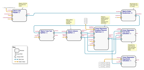
A basic linear regression workflow is defined by the XML document in 'SimpleML.Samples\Resources\Basic Linear Regression.xml'. The workflow first attempts to train a linear regression model providing historic market data of the ASX200 and Nikkei 225 indices as input features, and the corresponding exchange rate between the Australian Dollar and Japanese Yen as the result data. It then predicts the AUD/JPY exchange rate for 3 pairs of ASX200 and Nikkei 255 data values. A visual representation of the module graph for this workflow appears below (note that the bracketed numbers on each module correspond to the module id in the XML document). The training portion of the workflow is represented by the top two rows of modules. This training portion uses gradient descent to produce optimized theta parameters. These theta parameters are then used by the 'Linear Regression Hypothesis Calculator' module at the bottom right of the diagram to estimate the AUD/JPY exchange rate for the 3 pairs of data values.
The workflow can be executed by uncommenting the following code in the SimpleML.Samples.Program class, and running the sample project...
...and will result in the following output...
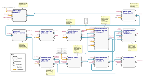
The results show as 'NaN' (not a number) because the gradient descent optimizer is not able to converge on optimized theta parameters (this can be confimed by switching on granular (debug) logging and looking at the intermediate cost values output by the gradient descent optimizer module). In order to achieve convergence, the feature data needs to be scaled to values between -1 and 1. The MMF framework supports this by allowing additional modules to be added the module graph to scale the input feature data, and then rescale the estimated results. Note that the modules carried over from the original workflow are unchanged. The updated workflow is defined by the XML document in 'SimpleML.Samples\Resources\Linear Regression with Feature Scaling.xml', and depicted below...
This workflow can be run by uncommenting the following code...
...and outputs the following data...
The estimated exchange rate values are as follows...
| ASX 200 Value | Nikkei 225 Value | Estimated AUD/JPY Exchange Rate |
|---|---|---|
| 5103.27 | 15323.14 | 89.57 |
| 5411.61 | 16385.89 | 92.37 |
| 3510.4 | 8235.87 | 76.51 |
Adding Polynomial Feature Generation
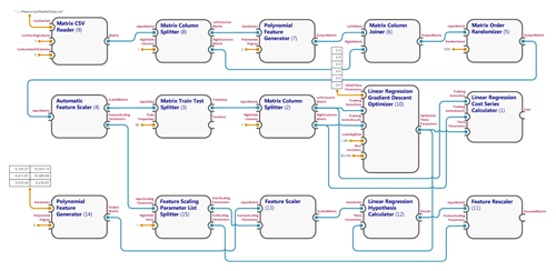
Greater accuracy can be achieved by generating polynomial features on the input data and using a higher order polynomial to interpolate it. The MMF framework supports this by allowing relevant polynomial feature generator modules to be added to the workflow. A corresponding module graph is defined in 'SimpleML.Samples\Resources\Linear Regression with Polynomial Features.xml' and is shown below...
'Polynomial Feature Generator' modules are applied to the input feature data (along the top row) and also to the 3 pairs of test data points (in the bottom left).
This workflow can be run by uncommenting the following code (note due to the much higher number of gradient descent iterations, this module graph may take up to a minute to execute)...
...and outputs the following data...
Note that the cost is lower, and the estimated exchange rate values differ to those of the workflow with no polynomial feature generation.
| ASX 200 Value | Nikkei 225 Value | Estimated AUD/JPY Exchange Rate |
|---|---|---|
| 5103.27 | 15323.14 | 89.15 |
| 5411.61 | 16385.89 | 91.67 |
| 3510.4 | 8235.87 | 72.86 |
Calculating the Cost Against the Test Data
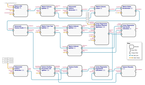
In all of the workflows analyzed so far, the module 'Matrix Train Test Splitter' has been used to split the input feature data into train and test portions, and the optimized theta parameters calculated from the train portion. In previous workflows, the cost incurred by the theta parameters (calculated by the 'Linear Regression Cost Series Calculator' module) was calculated against the train data. However to ensure the parameters improve the accuracy but do not overfit the feature data, the cost should be calculated against the test portion of the data. Again the MMF framework supports this by simply changing the SlotLinks in the module graph, and introducing one additional 'Matrix Column Splitter' module (to split the input and result data into separate matrices). The resulting module graphs for workflows with and without polynomial feature generation are defined in XML files 'SimpleML.Samples\Resources\Linear Regression with Polynomial Features and Test Data Cost.xml' and 'SimpleML.Samples\Resources\Linear Regression with Feature Scaling and Test Data Cost.xml'. The module graph for polynomial feature generation with the cost calculated against the test data is depicted below...
Comparing Workflows
The Workflow Comparison page provides a side-by-side comparison of the linear regression workflows described above.


